SPS Cavity Loop¶

Authors: Helga Timko

TRAVELLING WAVE CAVITY¶

The voltage in the SPS travelling-wave cavities (TWC) is the sum of the generator-induced voltage \(V_\mathsf{gen}\) and the beam-induced voltage \(V_\mathsf{beam}\),

\[V_\mathsf{ant} = V_\mathsf{gen} + V_\mathsf{beam} = I_\mathsf{gen} Z_\mathsf{gen} + I_\mathsf{beam} Z_\mathsf{beam}\, ,\]

where \(I\) represents currents and \(Z\) represent impedances. As shown by G. Dome, the impedance of the beam towards the TWC can be expressed as

\[Z_\mathsf{beam} (\omega) = \frac{\rho l^2}{8} \left[ \left( \frac{\sin \left(\frac{\tau(\omega - \omega_r)}{2}\right)}{\frac{\tau(\omega - \omega_r)}{2}} \right)^2 - 2i \frac{\tau(\omega - \omega_r) - \sin(\tau(\omega - \omega_r))}{(\tau(\omega - \omega_r))^2} + \left( \frac{\sin \left(\frac{\tau(\omega + \omega_r)}{2}\right)}{\frac{\tau(\omega + \omega_r)}{2}} \right)^2 + 2i \frac{\tau(\omega + \omega_r) - \sin(\tau(\omega + \omega_r))}{(\tau(\omega + \omega_r))^2} \right] \, .\]

Here, the TWC has the following properties:

\(\rho = 27.1 \frac{\mathsf{k\Omega}}{\mathsf{m}^2}\) is the series impedance
\(l = (11 n_\mathsf{sections} - 1) \times 0.374 \mathsf{m}\) is the accelerating length of the cavity, depending on the number of sections \(n_\mathsf{sections}\)
\(\tau = \frac{l}{v_g} \left( 1 + \frac{v_g}{c} \right)\) is the cavity filling time, where the group velocity is \(v_g = 0.0946 c\)
\(\omega_r = 200.222 \mathsf{MHz}\) is the resonant frequency of the TWC

The impedance of the generator towards the TWC is

\[Z_\mathsf{gen} (\omega) = l \sqrt{\frac{\rho Z_0}{2}} \left[ \frac{\sin \left(\frac{\tau(\omega - \omega_r)}{2}\right)}{\frac{\tau(\omega - \omega_r)}{2}} + \frac{\sin \left(\frac{\tau(\omega + \omega_r)}{2}\right)}{\frac{\tau(\omega + \omega_r)}{2}} \right] \, ,\]

where \(Z_0\) is the shunt impedance when measuring the generator current; assumed to be 50 \(\Omega\).

Induced-voltage calculation¶

In the discrete time system, the induced voltage \(V(t)\) is obtained from the impulse response \(h(t)\) and the complex (cavity or generator) current \(I(t)\), broken down to in-phase (I) and quadrature (Q) components. The induced-voltage calculation can be written in matrix form,

\[\begin{split}\left( \begin{matrix} V_I(t) \\ V_Q(t) \end{matrix} \right) = \left( \begin{matrix} h_s(t) & - h_c(t) \\ h_c(t) & h_s(t) \end{matrix} \right) * \left( \begin{matrix} I_I(t) \\ I_Q(t) \end{matrix} \right) \, ,\end{split}\]

where \(*\) denotes convolution, \(h(t)*x(t) = \int d\tau h(\tau)x(t-\tau)\).

Beam-induced voltage¶

For the voltage induced by the beam towards the TWC, we define the short-hand notation

\[R_\mathsf{beam} \equiv \frac{\rho l^2}{8} \, .\]

The beam-induced wake is

\[W_\mathsf{beam}(t) = \frac{4 R_\mathsf{beam}}{\tau} \mathsf{tri}\left(\frac{t}{\tau}\right) \cos(\omega_r t)\]

and the impulse response components are

\[\begin{split}h_{s,\mathsf{beam}}(t) &= \frac{2 R_\mathsf{beam}}{\tau} \mathsf{tri}\left(\frac{t}{\tau}\right) \cos((\omega_c - \omega_r)t) \, , \\ h_{c,\mathsf{beam}}(t) &= \frac{2 R_\mathsf{beam}}{\tau} \mathsf{tri}\left(\frac{t}{\tau}\right) \sin((\omega_c - \omega_r)t) \, ,\end{split}\]

where \(\mathsf{tri}(x)\) is the triangular function and \(\omega_c\) is the carrier revolution frequency of the I,Q demodulated current signal. On the resonant frequency of the cavity, \(\omega_c = \omega_r\),

\[\begin{split}h_{s,\mathsf{beam}}(t) &= \frac{2 R_\mathsf{beam}}{\tau} \mathsf{tri}\left(\frac{t}{\tau}\right) \\ h_{c,\mathsf{beam}}(t) &= 0 \, .\end{split}\]

Generator-induced voltage¶

For the voltage induced by the generator towards the TWC, we define

\[R_\mathsf{gen} \equiv l \sqrt{\frac{\rho Z_0}{2}} \, .\]

The generator-induced wake is

\[W_\mathsf{gen}(t) = \frac{2 R_\mathsf{gen}}{\tau} \mathsf{rect}\left(\frac{t}{\tau}\right)\cos(\omega_r t)\]

and the impulse-response components are

\[\begin{split}h_{s,\mathsf{gen}}(t) &= \frac{R_\mathsf{gen}}{\tau} \mathsf{rect}\left(\frac{t}{\tau}\right) \cos((\omega_c - \omega_r)t) \, , \\ h_{c,\mathsf{gen}}(t) &= \frac{R_\mathsf{gen}}{\tau} \mathsf{rect}\left(\frac{t}{\tau}\right) \sin((\omega_c - \omega_r)t) \, ,\end{split}\]

where \(\mathsf{rect}(x)\) is the rectangular function. On the resonant frequency of the TWC, \(\omega_c = \omega_r\),

\[\begin{split}h_{s,\mathsf{gen}}(t) &= \frac{R_\mathsf{gen}}{\tau} \mathsf{rect}\left(\frac{t}{\tau}\right) \\ h_{c,\mathsf{gen}}(t) &= 0 \, .\end{split}\]

THE CAVITY CONTROLLER¶

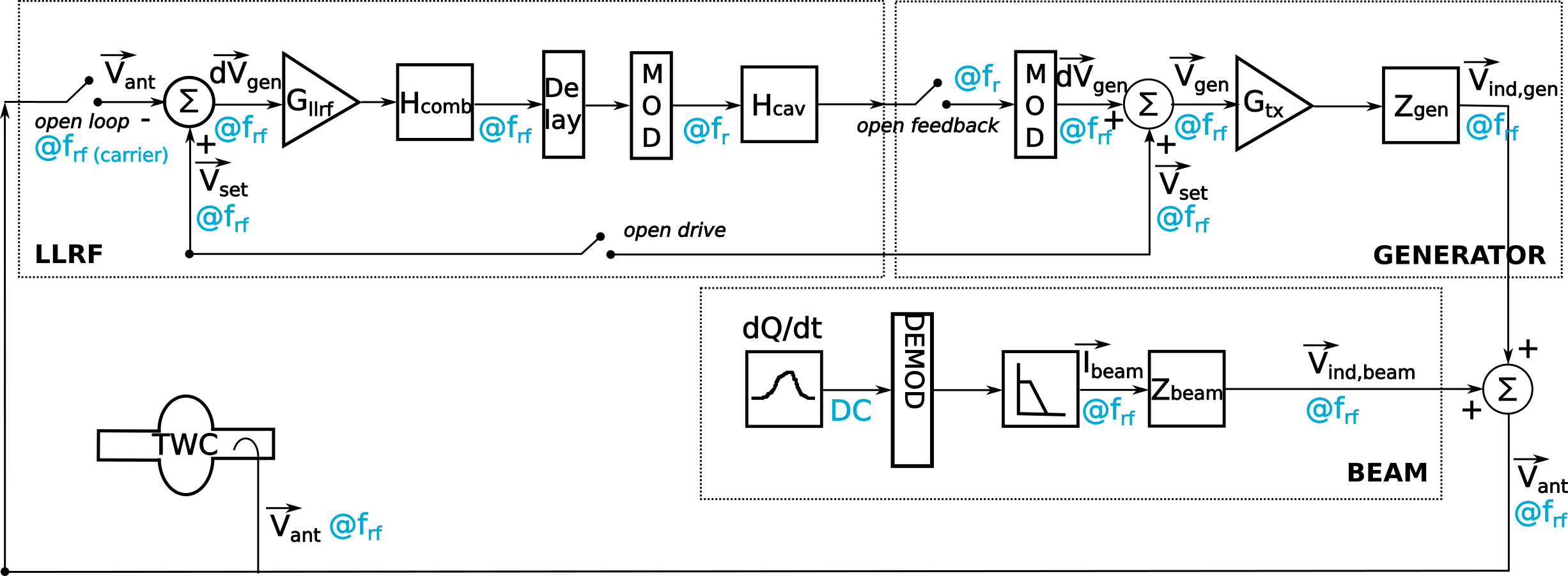
The cavity controller is a one-turn feedback, measuring in one turn and correcting in the turn after. It works on the carrier frequency of the present RF frequency \(f_{c}=f_{\mathsf{rf}}\). The cavity response is applied at the central or resonant frequency of the cavity \(f_{r}\), requiring and up- and down-modulation before and after. The controller loop is built of three entities in the code, see Figure.

Signal sampling¶

For beam particle tracking, the voltage amplitude and phase correction are calculated w.r.t.the values specified by the user in the RFStation object (voltage amplitude and phase set points). This correction is calculated on the time range and with the resolution of the beam Profile object; in the context of the cavity controller, we call it the fine grid.

The generator-induced voltage towards the cavity, as well as the low-level RF part are resolved on a bucket-by-bucket basis, which we call the coarse grid. The arrays cover the full ring, and keep in memory the previous turn for the tracking of the feedback. The sampling time \(T_s\) in turn \(n\) is defined as

\[T_{s,n} = T_{\mathsf{rf},n} \, ,\]

where \(T_{\mathsf{rf},n}\) is the RF period of the main RF system in the given turn. Arrays on the coarse grid have

\[n_{\mathsf{coarse}} \equiv \mathsf{int} \left( \frac{T_{\mathsf{rev},0}}{T_{\mathsf{rf},0}} \right)\]

sampling points, defined based on the initial revolution (\(T_{\mathsf{rev},0}\)) and RF periods. The centres of the sample number \(k\) along the time axis are

\[\mathsf{rf\_centers}_{k,n} = (i + \frac{1}{2}) T_{s,n} \, .\]

Note

When the RF frequency is not an integer multiple of the revolution frequency (as a result of the user declaring a non-harmonic RF frequency, or a beam feedback making a correction on the RF frequency, or both), a fraction of an RF period will be unsampled, and in the next turn, the RF signals are again sampled w.r.t. the beginning of the turn \(t_\mathsf{ref}\), as declared in the Equations of Motion. The non-harmonic RF frequency also results in the RF system \(s\) in an accumulated phase shift of

\[\sum_{i=1}^{n} \frac{\omega_{\mathsf{rf},s}^i - h_s^i \omega_0^i}{h_s^i \omega_0^i} 2 \pi h_s^i\]

between the signals of one turn to another. This phase shift is tracked in the blond.trackers.tracker; the the signal processing in the one-turn feedback, however, is performed w.r.t. the zero phase of the reference clock, and up- and down-modulation of (I,Q) signals does therefore not require a phase shift. In addition, the non-harmonic RF frequency can lead to a changing number of sampling points \(n_{\mathsf{coarse}}\) over time; this feature is presently not implemented in the SPS one-turn feedback and will thus result in a Runtime Error.

To pass information back and forth between the cavity controller and the voltage corrections to be applied, information from the coarse grid has to be interpolated to the fine grid, and information on the fine grid has to be evaluated also on the coarse grid.

Low-level RF¶

The low-level RF (LLRF) contains the comparison between the desired set-point voltage \(V_{\mathsf{set}}\) and the actual antenna voltage \(V_{\mathsf{ant}}\) in the travelling wave cavity (TWC), and acts on the difference \(dV_{\mathsf{gen}}=V_{\mathsf{set}}-V_{\mathsf{ant}}\) with the gain \(G_{\mathsf{llrf}}\). The comb filter \(H_{\mathsf{comb}}\) represents the LLRF filter that reduces the beam loading seen by the beam. It acts bunch by bunch, and with exactly one turn delay,

\[dV_{\mathsf{gen,out}, k, n} = a_{\mathsf{comb}} \, dV_{\mathsf{gen,out}, k, n-1} + (1 - a) \, dV_{\mathsf{gen,in}, k, n} \, ,\]

where \(V_{\mathsf{gen,in}}\) and \(V_{\mathsf{gen,out}}\) are at the input and output of the comb filter, respectively, \(k\) is the sample number along the ring (in time), and \(n\) is the index of the turn. The comb filter constant is \(a_{\mathsf{comb}}=15/16\) operationally. The output of the comb filter is filtered by the cavity response \(H_{\mathsf{cav}}\) represented as a moving average at 40~MS/s. The moving average over \(K\) points is

\[dV_{\mathsf{gen,out}, k} = \frac{1}{K} \sum_{i=k-K}^{k} dV_{\mathsf{gen,in}, i} \, .\]

Generator-induced voltage¶

On the generator branch, the transmitter gain \(G_\mathsf{tx}\) is applied and the voltage signal is converted into a charge distribution signal according to the transmitter model,

\[I_{\mathsf{gen}} = G_\mathsf{tx} \frac{V_{\mathsf{gen}}}{R_{\mathsf{gen}}} T_s \, ,\]

where the units are \([G_\mathsf{tx}] = 1\), \([V_\mathsf{gen}] = V\), \([R_\mathsf{gen}] = \Omega\), and \([T_s] = s\). The resulting charge distribution is given in \([I_{\mathsf{gen}}] = C\). The generator-induced voltage \(V_\mathsf{ind,gen}\) is then calculated from \(I_{\mathsf{gen}}\) with the matrix convolution through the generator impulse response, as explained above in Generator-induced voltage.

Both the voltage and the current are calculated on the coarse grid.

Beam-induced voltage¶

On the beam-induced voltage branch, the beam profile is used as an input to calculate the RF component of the beam current, \(I_{\mathsf{beam}}\). Just like on the generator branch, this complex (I,Q) current is then matrix- convolved with the beam response, as described in Beam-induced voltage, to obtain the beam-induced voltage \(V_\mathsf{ind,beam}\).

The voltage and the current are calculated both on the fine and the coarse grid.

From coarse to fine grid and back¶

For beam particle tracking, the voltage amplitude and phase correction w.r.t.the set point values is applied on the grid of the beam profile, slice by slice. In order to calculate this correction, the generator-induced voltage is interpolated to the fine grid, and added to the beam-induced voltage already evaluated on the fine grid.

To track the SPS one-turn feedback itself, the generator- and beam-induced voltages are summed on the coarse grid that covers the entire turn,

\[V_\mathsf{ant} = V_\mathsf{ind,gen} + V_\mathsf{ind,beam} \, .\]

Feed-forward¶

Optionally, an n-tap FIR filter can be activated as feed-forward on the beam-induced voltage calculation. The feed-forward is used in open loop, to correct the generator current in the next turn based on the beam-induced voltage measured in the current turn. The ideal feed-forward filter \(H_\mathsf{FF}\) would perfectly compensate the beam loading if

\[Z_\mathsf{gen}(f) H_\mathsf{FF}(f) = - Z_\mathsf{beam}(f) \, .\]

The FIR filters for the 3-, 4-, 5-section cavities are designed by minimising the error between these two quantities, using the least-squares method and the FIR filter coefficients can be found in blond.llrf.signal_processing.