llrf Package

notch_filter Module

Method to apply a notch filter to a specified impedance source

Authors

Danilo Quartullo

blond.llrf.notch_filter.impedance_notches(f_rev, frequencies, imp_source, list_harmonics, list_width_depth)

llrf.beam_feedback Module

Various beam phase loops (PL) with optional synchronisation (SL), frequency (FL), or radial loops (RL) for the CERN machines

Authors

Helga Timko

Machine-dependent Beam Phase Loop

class llrf.phase_loop.PhaseLoop(object).__init__(GeneralParameters, RFSectionParameters, Slices, gain, gain2 = 0, machine = 'LHC', period = None, window_coefficient = 0, coefficients = None, PhaseNoise = None, LHCNoiseFB = None)

One-turn PL for different machines with different hardware. The beam phase is calculated as the convolution of the beam profile with the RF wave of the main harmonic system (corresponding to a band-pass filter). The PL acts directly on the RF frequency and phase of all harmonics.

Some machine-dependent features:

• PSB: use sampling_frequency for a PL that is active only at certain turns.

• SPS: use window coefficient to sample beam phase over a suitable amount of bunches (window_coefficient = 0 results in single-bunch acquisition as in the LHC)

• LHC_F: PL with optional FL (use gain2 to activate)

• LHC: PL with optional SL (use gain2 to activate; note that gain is frequency dependent)

Parameters

• GeneralParameters – input_parameters.general_parameters.GeneralParameters

• RFSectionParameters – input_parameters.rf_parameters.RFSectionParameters

• Slices – beams.slices.Slices

• gain (double) – phase loop gain [1/ns], typically \(\sim 1/(10 T_0)\)

• gain2 (double) – FL gain [turns] or SL gain [1/ns], depending on machine; typically ~10 times weaker than PL

• machine (str) – machine name, determines PL choice

• period (double) – optional for PSB: period of PL being active

• window_coefficient (double) – window coefficient for band-pass filter determining beam phase; use 0 for single-bunch acquisition

• coefficients (array) – optional for PSB: PL transfer function coefficients

• PhaseNoise – optional: phase-noise type class for noise injection through the PL, llrf.rf_noise.PhaseNoise or llrf.rf_noise.LHCFlatSpectrum

• LHCNoiseFB – optional: bunch-length feedback class for phase noise llrf.rf_noise.LHCNoiseFB

track()

Calculates the PL correction on main RF frequency depending on machine. Updates the RF phase and frequency of the next turn for all RF systems.

Let \(\Delta \omega_{\mathsf{TOT}}\) be the total frequency correction (calculation depends on the machine, see below). The RF frequency of a given RF system \(i\) is then shifted by

\[\Delta \omega_{\mathsf{rf},i} = \frac{h_i}{h_0} \Delta \omega_{\mathsf{TOT}} ,\]

with a corresponding RF phase shift of

\[\Delta \varphi_{\mathsf{rf},i} = 2 \pi h_i \frac{\omega_{\mathsf{rf},i}}{\Omega_{\mathsf{rf},i}} ,\]

where \(\Omega_{\mathsf{rf},i} = h_i \omega_0\) is the design frequency and \(\omega_{\mathsf{rf},i}\) the actual RF frequency applied.

precalculate_time(GeneralParameters)

For PSB, where the PL acts only with a given periodicity, pre-calculate on which turns to act.

Parameters

GeneralParameters – input_parameters.general_parameters.GeneralParameters

beam_phase()

Beam phase measured at the main RF frequency and phase. The beam is convolved with the window function of the band-pass filter of the machine. The coefficients of sine and cosine components determine the beam phase, projected to the range -Pi/2 to 3/2 Pi.

Note

that this beam phase is already determined w.r.t. the instantaneous RF phase.

The band-pass filter modelled assumes a window function of the form

\[W(t) = e^{-\alpha t} \cos(\omega_{\mathsf{rf}} t - \varphi_{\mathsf{rf}}) ,\]

where \(\alpha\) is the window_coefficient that determines how many bunches are taken into account.

The convolution of \(W(t)\) with the bunch profile \(\lambda(t)\) results in two components,

\[f(t) = \int_{\lambda_{\mathsf{min}}}^{\lambda_{\mathsf{max}}} {e^{-\alpha (t-\tau)} \cos(\omega_{\mathsf{rf}} (t-\tau) - \varphi_{\mathsf{rf}}) \lambda(\tau) d\tau} = e^{-\alpha t} \cos(\omega_{\mathsf{rf}} t) \int_{\lambda_{\mathsf{min}}}^{\lambda_{\mathsf{max}}} {e^{\alpha \tau} \cos(\omega_{\mathsf{rf}} \tau + \varphi_{\mathsf{rf}}) \lambda(\tau) d\tau} + e^{-\alpha t} \sin(\omega_{\mathsf{rf}} t) \int_{\lambda_{\mathsf{min}}}^{\lambda_{\mathsf{max}}} {e^{\alpha \tau} \sin(\omega_{\mathsf{rf}} \tau + \varphi_{\mathsf{rf}}) \lambda(\tau) d\tau} .\]

The beam phase is determined from the coefficients of the sine and cosine components, i.e.

\[\varphi_b \equiv \arctan \left( \frac{\int_{\lambda_{\mathsf{min}}}^{\lambda_{\mathsf{max}}} {e^{\alpha \tau} \sin(\omega_{\mathsf{rf}} \tau + \varphi_{\mathsf{rf}}) \lambda(\tau) d\tau}} {\int_{\lambda_{\mathsf{min}}}^{\lambda_{\mathsf{max}}} {e^{\alpha \tau} \cos(\omega_{\mathsf{rf}} \tau + \varphi_{\mathsf{rf}}) \lambda(\tau) d\tau}} \right) .\]

This projects the beam phase to the interval \(\left( -\frac{\pi}{2} , \frac{\pi}{2}\right)\), however, the RF phase is defined on the interval \(\left( -\frac{\pi}{2} , \frac{3 \pi}{2}\right)\). In order to get a correct measurement of the beam phase, we thus add \(\pi\) if the cosine coefficient is negative (meaning normally the beam energy is above transition).

phase_difference()

Phase difference between beam and RF phase of the main RF system. Optional: add RF phase noise through dphi directly.

As the actual RF phase is taken into account already in the beam phase calculation, only the synchronous phase needs to be substracted and thus the phase difference seen by the PL becomes

\[\Delta \varphi_{\mathsf{PL}} = \varphi_b - \varphi_s .\]

If phase noise is injected through the PL, it is added directly as an offset to this measurement, optionally with the feedback scaling factor \(x\).

\[\Delta \varphi_{\mathsf{PL}} = \varphi_b - \varphi_s + (x) \phi_N .\]

LHC_F():

Calculates the RF frequency correction \(\Delta \omega_{\mathsf{PL}}\) from the phase difference between beam and RF \(\Delta \varphi_{\mathsf{PL}}\) for the LHC. The transfer function is

\[\Delta \omega_{\mathsf{PL}} = - g_{\mathsf{PL}} \Delta\varphi_{\mathsf{PL}} ,\]

Using ‘gain2’, the frequency loop can be activated in addition to remove long-term frequency drifts:

\[\Delta \omega_{\mathsf{FL}} = - g_{\mathsf{FL}} (\omega_{\mathsf{rf}} - h \omega_{0}) .\]

LHC()

Calculates the RF frequency correction \(\Delta \omega_{\mathsf{PL}}\) from the phase difference between beam and RF \(\Delta \varphi_{\mathsf{PL}}\) for the LHC. The transfer function is

\[\Delta \omega_{\mathsf{PL}} = - g_{\mathsf{PL}} \Delta \varphi_{\mathsf{PL}} ,\]

Using ‘gain2’, a synchro loop can be activated in addition to remove long-term frequency and phase drifts:

\[\Delta \omega_{\mathsf{SL}} = - g_{\mathsf{SL}} (y + a \, \Delta \varphi_{\mathsf{rf}}) ,\]

where \(\Delta \varphi_{\mathsf{rf}}\) is the accumulated RF phase deviation from the design value and \(y\) is is obtained through the recursion (\(y_0 = 0\))

\[y_{n+1} = (1 - \tau) y_n + (1 - a) \tau \Delta \varphi_{\mathsf{rf}} .\]

The variables \(a\) and \(\tau\) are being defined through the (single-harmonic, central) synchrotron frequency \(f_s\) and the corresponding synchrotron tune \(Q_s\) as

\[a (f_s) \equiv 5.25 - \frac{f_s}{\pi 40~\text{Hz}} ,\]

\[\tau(f_s) \equiv 2 \pi Q_s \sqrt{ \frac{a}{1 + \frac{g_{\mathsf{PL}}}{g_{\mathsf{SL}}} \sqrt{\frac{1 + 1/a}{1 + a}} }} .\]

PSB():

Phase loop:

The transfer function of the system is

\[H(z) = g \frac{b_{0}+b_{1} z^{-1}}{1 +a_{1} z^{-1}}\]

where g is the gain and \(b_{0} = 0.99901903\), \(b_{1} = -0.99901003\), \(a_{1} = -0.99803799\).

Let \(\Delta \phi_{PL}\) and \(\Delta \omega_{PL}\) be the phase difference and the phase loop correction on the frequency respectively; since these two quantities are the input and output of our system, then from the transfer function we have in time domain (see https://en.wikipedia.org/wiki/Z-transform):

\[\Delta \omega_{PL}^{n+1} = - a_{1} \Delta \omega_{PL}^{n} + g(b_{0} \Delta \phi_{PL}^{n+1} + b_{1} \Delta \phi_{PL}^{n})\]

In fact the phase and radial loops act every 10 \(\mu s\) and as a consequence \(\Delta \phi_{PL}\) is an average on all the values between two trigger times.

Radial loop:

We estimate the difference of the radii of the actual trajectory and the desired trajectory using one of the four known differential relations with \(\Delta B = 0\):

\[\frac{\Delta R}{R} = \frac{\Delta \omega_{RF}}{\omega_{RF}} \frac{\gamma^2}{\gamma_{T}^2-\gamma^2}\]

In reality the error \(\Delta R\) is filtered with a PI (Proportional- Integrator) corrector. This means that

\[\Delta \omega_{RL}^{n+1} = K_{P} \left(\frac{\Delta R}{R}\right)^{n} + K_{I} \int_0^n \! \frac{\Delta R}{R} (t) \, \mathrm{d}t.\]

Writing the same equation for \(\Delta \omega_{RL}^{n}\) and subtracting side by side we have

\[\Delta \omega_{RL}^{n+1} = \Delta \omega_{RL}^{n} + K_{P} \left[ \left(\frac{\Delta R}{R}\right)^{n} - \left(\frac{\Delta R}{R}\right)^{n-1} \right] + K_{I}^{'} \left(\frac{\Delta R}{R}\right)^{n}\]

here \(K_{I}^{'} = K_{I} 10 \mu s\) and we approximated the integral with a simple product.

The total correction is then

\[\Delta \omega_{RF}^{n+1} = \Delta \omega_{PL}^{n+1} + \Delta \omega_{RL}^{n+1}\]

cavity_feedback Module

Various cavity loops for the CERN machines

Authors

Helga Timko

class blond.llrf.cavity_feedback.CavityFeedbackCommissioning(debug=False, open_loop=False, open_FB=False, open_drive=False, open_FF=False)

Bases: object

class blond.llrf.cavity_feedback.SPSCavityFeedback(RFStation, Beam, Profile, G_ff=1, G_llrf=10, G_tx=0.5, a_comb=0.9375, turns=1000, post_LS2=True, V_part=None, Commissioning=<blond.llrf.cavity_feedback.CavityFeedbackCommissioning object>)

Bases: object

Class determining the turn-by-turn total RF voltage and phase correction originating from the individual cavity feedbacks. Assumes two 4-section and two 5-section travelling wave cavities in the pre-LS2 scenario and four 3-section and two 4-section cavities in the post-LS2 scenario. The voltage partitioning is proportional to the number of sections.

Parameters

• RFStation (class) – An RFStation type class

• Beam (class) – A Beam type class

• Profile (class) – A Profile type class

• G_llrf (float or list) – LLRF Gain [1]; if passed as a float, both 3- and 4-section (4- and 5-section) cavities have the same G_llrf in the post- (pre-)LS2 scenario. If passed as a list, the first and second elements correspond to the G_llrf of the 3- and 4-section (4- and 5-section) cavity feedback in the post- (pre-)LS2 scenario; default is 10

• G_tx (float or list) – Transmitter gain [1] of the cavity feedback; convention same as G_llrf; default is 0.5

• a_comb (float) – Comb filter ratio [1]; default is 15/16

• turns (int) – Number of turns to pre-track without beam

• post_LS2 (bool) – Activates pre-LS2 scenario (False) or post-LS2 scenario (True); default is True

• V_part (float) – Voltage partitioning of the shorter cavities; has to be in the range (0,1). Default is None and will result in 6/10 for the 3-section cavities in the post-LS2 scenario and 4/9 for the 4-section cavities in the pre-LS2 scenario

OTFB_1

An SPSOneTurnFeedback type class; 3/4-section cavity for post/pre-LS2

Type

class

OTFB_2

An SPSOneTurnFeedback type class; 4/5-section cavity for post/pre-LS2

Type

class

V_sum

Vector sum of RF voltage from all the cavities

Type

complex array

V_corr

RF voltage correction array to be applied in the tracker

Type

float array

phi_corr

RF phase correction array to be applied in the tracker

Type

float array

logger

Logger of the present class

Type

logger

track()

track_init(debug=False)

Tracking of the SPSCavityFeedback without beam.

class blond.llrf.cavity_feedback.SPSOneTurnFeedback(RFStation, Beam, Profile, n_sections, n_cavities=2, V_part=0.4444444444444444, G_ff=1, G_llrf=10, G_tx=0.5, a_comb=0.9375, Commissioning=<blond.llrf.cavity_feedback.CavityFeedbackCommissioning object>)

Bases: object

Voltage feedback around a travelling wave cavity with given amount of sections. The quantities of the LLRF system cover one turn with a coarse resolution.

Parameters

• RFStation (class) – An RFStation type class

• Beam (class) – A Beam type class

• Profile (class) – Beam profile object

• n_sections (int) – Number of sections in the cavities

• n_cavities (int) – Number of cavities of the same type

• V_part (float) – Voltage partition for the given n_cavities; in range (0,1)

• G_ff (float) – FF gain [1]; default is 1

• G_llrf (float) – LLRF gain [1]; default is 10

• G_tx (float) – Transmitter gain [A/V]; default is \((50 \Omega)^{-1}\)

• open_loop (int(bool)) – Open (0) or closed (1) feedback loop; default is 1

TWC

A TravellingWaveCavity type class

Type

class

counter

Counter of the current time step

Type

int

omega_c

Carrier revolution frequency [1/s] at the current time step

Type

float

omega_r

Resonant revolution frequency [1/s] of the travelling wave cavities

Type

const float

n_coarse

Number of bins for the coarse grid (equals harmonic number)

Type

int

V_gen

Generator voltage [V] of the present turn in (I,Q) coordinates

Type

complex array

V_gen_prev

Generator voltage [V] of the previous turn in (I,Q) coordinates

Type

complex array

V_fine_ind_beam

Beam-induced voltage [V] in (I,Q) coordinates on the fine grid used for tracking the beam

Type

complex array

V_coarse_ind_beam

Beam-induced voltage [V] in (I,Q) coordinates on the coarse grid used tracking the LLRF

Type

complex array

V_coarse_ind_gen

Generator-induced voltage [V] in (I,Q) coordinates on the coarse grid used tracking the LLRF

Type

complex array

V_coarse_tot

Cavity voltage [V] at present turn in (I,Q) coordinates which is used for tracking the LLRF

Type

complex array

V_fine_tot

Cavity voltage [V] at present turn in (I,Q) coordinates which is used for tracking the beam

Type

complex array

a_comb

Recursion constant of the comb filter; \(a_{\mathsf{comb}}=15/16\)

Type

float

n_mov_av

Number of points for moving average modelling cavity response; \(n_{\mathsf{mov.av.}} = \frac{f_r}{f_{\mathsf{bw,cav}}}\), where \(f_r\) is the cavity resonant frequency of TWC_4 and TWC_5

Type

const int

logger

Logger of the present class

Type

logger

beam_induced_voltage(lpf=False)

Calculates the beam-induced voltage

Parameters

lpf (bool) – Apply low-pass filter for beam current calculation; default is False

I_beam_coarse

RF component of the beam charge [C] at the present time step, calculated in coarse grid

Type

complex array

I_beam_fine

RF component of the beam charge [C] at the present time step, calculated in fine grid

Type

complex array

V_coarse_ind_beam

Induced voltage [V] from beam-cavity interaction on the coarse grid

Type

complex array

V_fine_ind_beam

Induced voltage [V] from beam-cavity interaction on the fine grid

Type

complex array

call_conv(signal, kernel)

Routine to call optimised C++ convolution

generator_induced_voltage()

Calculates the generator-induced voltage. The transmitter model is a simple linear gain [C/V] converting voltage to charge.

\[I = G_{\mathsf{tx}}\,\frac{V}{R_{\mathsf{gen}}} \, ,\]

where \(R_{\mathsf{gen}}\) is the generator resistance, llrf.impulse_response.TravellingWaveCavity.R_gen

I_gen

RF component of the generator charge [C] at the present time step

Type

complex array

V_coarse_ind_gen

Induced voltage [V] from generator-cavity interaction

Type

complex array

induced_voltage(name)

Generation of beam- or generator-induced voltage from the beam or generator current, at a given carrier frequency and turn. The induced voltage \(V(t)\) is calculated from the impulse response matrix \(h(t)\) as follows:

\[\begin{split}\left( \begin{matrix} V_I(t) \\ V_Q(t) \end{matrix} \right) = \left( \begin{matrix} h_s(t) & - h_c(t) \\ h_c(t) & h_s(t) \end{matrix} \right) * \left( \begin{matrix} I_I(t) \\ I_Q(t) \end{matrix} \right) \, ,\end{split}\]

where \(*\) denotes convolution, \(h(t)*x(t) = \int d\tau h(\tau)x(t-\tau)\). If the carrier frequency is close to the cavity resonant frequency, \(h_c = 0\).

See also

llrf.impulse_response.TravellingWaveCavity

The impulse response is made to be the same length as the beam profile.

llrf_model()

Models the LLRF part of the OTFB.

V_set

Voltage set point [V] in (I,Q); \(V_{\mathsf{set}}\), amplitude proportional to voltage partition

Type

complex array

dV_gen

Generator voltage [V] in (I,Q); \(dV_{\mathsf{gen}} = V_{\mathsf{set}} - V_{\mathsf{tot}}\)

Type

complex array

matr_conv(I, h)

Convolution of beam current with impulse response; uses a complete matrix with off-diagonal elements.

track()

Turn-by-turn tracking method.

track_no_beam()

Initial tracking method, before injecting beam.

update_variables()

Update counter and frequency-dependent variables in a given turn

impulse_response Module

Filters and methods for control loops

Authors

Helga Timko

class blond.llrf.impulse_response.SPS3Section200MHzTWC

Bases: blond.llrf.impulse_response.TravellingWaveCavity

class blond.llrf.impulse_response.SPS4Section200MHzTWC

Bases: blond.llrf.impulse_response.TravellingWaveCavity

class blond.llrf.impulse_response.SPS5Section200MHzTWC

Bases: blond.llrf.impulse_response.TravellingWaveCavity

class blond.llrf.impulse_response.TravellingWaveCavity(l_cell, N_cells, rho, v_g, omega_r)

Bases: object

Impulse responses of a travelling wave cavity. The induced voltage \(V(t)\) from the impulse response \(h(t)\) and the I,Q (cavity or generator) current \(I(t)\) can be written in matrix form,

\[\begin{split}\left( \begin{matrix} V_I(t) \\ V_Q(t) \end{matrix} \right) = \left( \begin{matrix} h_s(t) & - h_c(t) \\ h_c(t) & h_s(t) \end{matrix} \right) * \left( \begin{matrix} I_I(t) \\ I_Q(t) \end{matrix} \right) \, ,\end{split}\]

where \(*\) denotes convolution, \(h(t)*x(t) = \int d\tau h(\tau)x(t-\tau)\).

For the cavity-to-beam induced voltage, we define

\[R_b \equiv \frac{\rho l^2}{8} \,\]

where \(\rho\) is the series impedance, \(l\) the accelerating length, \(\tau\) the filling time. The cavity-to-beam wake is

\[W_b(t) = \frac{4 R_b}{\tau} \mathsf{tri}\left(\frac{t}{\tau}\right) \cos(\omega_r t)\]

and the impulse response components are

\[\begin{split}h_{s,b}(t) &= \frac{2 R_b}{\tau} \mathsf{tri}\left(\frac{t}{\tau}\right) \cos((\omega_c - \omega_r)t) \, , \\ h_{c,b}(t) &= \frac{2 R_b}{\tau} \mathsf{tri}\left(\frac{t}{\tau}\right) \sin((\omega_c - \omega_r)t) \, ,\end{split}\]

where \(\mathsf{tri}(x)\) is the triangular function, \(\omega_r\) is the central revolution frequency of the cavity, and \(\omega_c\) is the carrier revolution frequency of the I,Q demodulated current signal. On the carrier frequency, \(\omega_c = \omega_r\),

\[\begin{split}h_{s,b}(t) &= \frac{2 R_b}{\tau} \mathsf{tri}\left(\frac{t}{\tau}\right) \\ h_{c,b}(t) &= 0 \, .\end{split}\]

For the cavity-to-generator induced voltage, we define

\[R_g \equiv l \sqrt{\frac{\rho Z_0}{2}} \,\]

where \(Z_0\) is the shunt impedance when measuring the generator current; assumed to be 50 \(\Omega\). The cavity-to-generator wake is

\[W_g(t) = \frac{2 R_g}{\tau} \mathsf{rect}\left(\frac{t}{\tau}\right) \cos(\omega_r t)\]

and the impulse response components are

\[\begin{split}h_{s,g}(t) &= \frac{R_g}{\tau} \mathsf{rect}\left(\frac{t}{\tau}\right) \cos((\omega_c - \omega_r)t) \, , \\ h_{c,g}(t) &= \frac{R_g}{\tau} \mathsf{rect}\left(\frac{t}{\tau}\right) \sin((\omega_c - \omega_r)t) \, ,\end{split}\]

where \(\mathsf{rect}(x)\) is the rectangular function. On the carrier frequency, \(\omega_c = \omega_r\),

\[\begin{split}h_{s,g}(t) &= \frac{R_g}{\tau} \mathsf{rect}\left(\frac{t}{\tau}\right) \\ h_{c,g}(t) &= 0 \, .\end{split}\]

Parameters

• l_cell (float) – Cavity cell length [m]

• N_cells (int) – Number of accelerating (interacting) cells in a cavity

• rho (float) – Series impedance [Ohms/m^2] of the cavity

• v_g (float) – Group velocity [c] in units of the speed of light

• omega_r (flaot) – Central (resonance) revolution frequency [1/s] of the cavity

Z_0

Shunt impedance of generator current measurement; assumed to be 50 Ohms

Type

float

R_beam

\(R_b\) [Omega] as defined above

Type

float

R_gen

\(R_g\) [Omega] as defined above

Type

float

l_cav

Length [m] of the interaction region

Type

float

tau

Cavity filling time [s]

Type

float

compute_wakes(time)

Computes the wake fields towards the beam and generator on the central cavity frequency.

Parameters

• time_beam (float) – Time array of the beam to act on

• time_gen (float) – Time array of the generator to act on

W_beam

\(W_b(t)\) [Omega/s] as defined above

Type

float array

W_gen

\(W_g(t)\) [Omega/s] as defined above

Type

float array

impulse_response_beam(omega_c, time_fine, time_coarse=None)

Impulse response from the cavity towards the beam. For a signal that is I,Q demodulated at a given carrier frequency \(\omega_c\). The formulae assume that the carrier frequency is be close to the central frequency \(\omega_c/\omega_r \ll 1\) and that the signal is low-pass filtered (i.e.high-frequency components can be neglected).

Parameters

• omega_c (float) – Carrier revolution frequency [1/s]

• time_fine (float) – Time array of the beam profile to act on

• time_coarse (float) – Time array of the LLRF to act on; default is None

d_omega

\(\omega_c - \omega_r\) [1/s]

Type

float

t_beam

time array for beam wake and impulse response; starts from zero

Type

float array

h_beam

\(h_{s,b}(t) + i*h_{c,b}(t)\) [Omega/s] as defined above

Type

complex array

h_beam_coarse

Impulse response evaluated on the coarse grid

Type

complex array

impulse_response_gen(omega_c, time_coarse)

Impulse response from the cavity towards the generator. For a signal that is I,Q demodulated at a given carrier frequency \(\omega_c\). The formulae assume that the carrier frequency is be close to the central frequency \(\omega_c/\omega_r \ll 1\) and that the signal is low-pass filtered (i.e.high-frequency components can be neglected).

Parameters

• omega_c (float) – Carrier revolution frequency [1/s]

• time_coarse (float) – Time array of the LLRF to act on

d_omega

\(\omega_c - \omega_r\) [1/s]

Type

float

t_gen

time array for generator wake and impulse response; starts from \(- \tau/2\)

Type

float array

h_gen

\(h_{s,b}(t) + i*h_{c,b}(t)\) [Omega/s] as defined above

Type

complex array

blond.llrf.impulse_response.rectangle(t, tau)

Rectangular function of time

\[\begin{split}\mathsf{rect} \left( \frac{t}{\tau} \right) = \begin{cases} 1 \, , \, t \in (-\tau/2, \tau/2) \\ 0.5 \, , \, t = \pm \tau/2 \\ 0 \, , \, \textsf{otherwise} \end{cases}\end{split}\]

Parameters

• t (float array) – Time array

• tau (float) – Time window of rectangular function

Returns

Rectangular function for given time array

Return type

float array

blond.llrf.impulse_response.triangle(t, tau)

Triangular function of time

\[\begin{split}\mathsf{tri} \left( \frac{t}{\tau} \right) = \begin{cases} 1 - \frac{t}{\tau}\, , \, t \in (0, \tau) \\ 0.5 \, , \, t = 0 \\ 0 \, , \, \textsf{otherwise} \end{cases}\end{split}\]

Parameters

• t (float array) – Time array

• tau (float) – Time window of rectangular function

Returns

Triangular function for given time array

Return type

float array

rf_modulation Module

Methods to generate RF phase modulation from given frequency, amplitude and offset functions

Authors

Simon Albright

class blond.llrf.rf_modulation.PhaseModulation(timebase, frequency, amplitude, offset, harmonic, multiplier=1, modulate_frequency=True)

Bases: object

calc_delta_omega(omegaProg)

calc_modulation()

extend_to_n_rf(harmonics)

llrf.rf_noise Module

Methods to generate RF phase noise from noise spectrum and feedback noise amplitude as a function of bunch length

Authors

Helga Timko

RF phase noise generation

class llrf.rf_noise.PhaseNoise(object).__init__(frequency_array, real_part_of_spectrum, seed1=None, seed2=None)

Contains the spectrum of RF phase noise and the actual phase noise randomly generated from it. Generation done via mixing with white noise.

Parameters

• frequency_array (numpy.array) – input frequency range

• real_part_of_spectrum (numpy.array) – input spectrum, real part only, same length as frequency_array

• seed1 (int) – seed for random number generator

• seed2 (int) – seed for random number generator

Warning

The spectrum has to be input as double-sided spectrum, in units of [\(\text{rad}^2/\text{Hz}\)].

Both hermitian to real and complex to complex FFTs are available. Use seeds to fix a certain random number sequence; with seed=None a random sequence will be initialized.

spectrum_to_phase_noise(transform=None)

Transforms a noise spectrum to phase noise data.

Parameters

transform (choice) – FFT transform kind

Returns

time and phase noise arrays

Note

Use transform=None or 'r' to transform hermitian spectrum to real phase. In this case, input only the positive part of the double-sided spectrum. Use transform='c' to transform complex spectrum to complex phase. In this case, input first the zero and positive frequency components, then the decreasingly negative frequency components of the double-sided spectrum. Returns only the real part of the phase noise. E.g. the following two ways of usage are equivalent: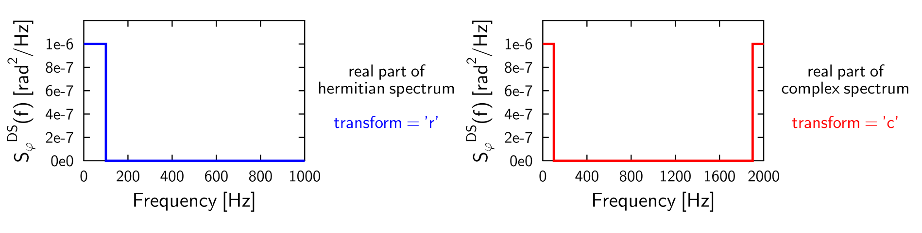

The transformation in steps

Step 1: Set the resolution in time domain. To transform a hermitian spectrum to real phase noise,

\[n_t = 2 (n_f - 1) \text{\,\,and\,\,} \Delta t = 1/(2 f_{\text{max}}) ,\]

and to transform a complex spectrum to complex phase noise,

\[n_t = n_f \text{\,\,and\,\,} \Delta t = 1/f_{\text{max}} ,\]

where fmax is the maximum frequency in the input in both cases.

Step 2: Generate white (carrier) noise in time domain

\[ \begin{align}\begin{aligned}w_k(t) = \cos(2 \pi r_k^{(1)}) \sqrt{-2 \ln(r_k^{(2)})} \text{\,\,\,case `r'},\\w_k(t) = \exp(2 \pi i r_k^{(1)}) \sqrt{-2 \ln(r_k^{(2)})} \text{\,\,\,case `c'},\end{aligned}\end{align} \]

Step 3: Transform the generated white noise to frequency domain

\[W_l(f) = \sum_{k=1}^N w_k(t) e^{-2 \pi i \frac{k l}{N}} .\]

Step 4: In frequency domain, colour the white noise with the desired noise probability density (unit: radians). The noise probability density derived from the double-sided spectrum is

\[s_l(f) = \sqrt{A S_l^{\text{DB}} f_{\text{max}}} ,\]

where \(A=2\) for transform = 'r' and \(A=1\) for transform = 'c'. The coloured noise is obtained by multiplication in frequency domain

\[\Phi_l(f) = s_l(f) W_l(f) .\]

Step 5: Transform back the coloured spectrum to time domain to obtain the final phase shift array (we use only the real part).

LHC-type phase noise generation

class llrf.rf_noise.LHCFlatSpectrum(object).__init__(GeneralParameters, RFSectionParameters, time_points, corr_time = 10000, fmin = 0.8571, fmax = 1.1, initial_amplitude = 1.e-6, seed1 = 1234, seed2 = 7564)

Generates LHC-type phase noise from a band-limited spectrum. Input frequency band using fmin and fmax w.r.t. the synchrotron frequency. Input double-sided spectrum amplitude [\(\text{rad}^2/\text{Hz}\)] using initial_amplitude. Fix seeds to obtain reproducible phase noise. Select time_points suitably to resolve the spectrum in frequency domain. After corr_time turns, the seed is changed (reproducibly) to cut numerical correlated sequences of the random number generator.

Parameters

• GeneralParameters – input_parameters.general_parameters.GeneralParameters

• RFSectionParameters – input_parameters.rf_parameters.RFSectionParameters

• time_points (int) – number of phase noise points of a sample in time domain

• corr_time (int) – number of turns after which seed is changed

• fmin (double) – spectrum lower limit in units of synchrotron frequency

• fmax (double) – spectrum upper limit in units of synchrotron frequency

• initial_amplitude (double) – initial double sided spectral density [\(\text{rad}^2/\text{Hz}\)]

• seed1 (int) – seed for random number generator

• seed2 (int) – seed for random number generator

Warning

time_points should be chosen large enough to resolve the desired frequency step \(\Delta f =\) GeneralParameters.f_rev/LHCFlatSpectrum.time_points in frequency domain.

generate()

Generates LHC-type phase noise array (length: GeneralParameters.n_turns + 1). Stored in the variable LHCFlatSpectrum.dphi.

Bunch-length based feedback on noise amplitude

class llrf.rf_noise.LHCNoiseFB(object).__init__(bl_target, gain = 1.5, factor = 0.8)

Feedback on phase noise amplitude for LHC controlled longitudinal emittance blow-up using noise injection through cavity controller or phase loop. The feedback compares the FWHM bunch length of the bunch to a target value and scales the phase noise to keep the targeted value.

Parameters

• bl_target – Targeted 4-sigma-equivalent FWHM bunch length [ns]

• gain – feedback gain [1/ns]

• factor – feedback recursion scaling factor [1]

Warning

Note that the FWMH bunch length is scaled by \(\sqrt{2/\ln{2}}\) in order to obtain a 4-sigma equivalent value.

FB(RFSectionParameters, Beam, PhaseNoise, Slices, CC=False)

Calculates the bunch-length based feedback scaling factor as a function of measured FWHM bunch length. For phase noise injected through the cavity RF voltage, the feedback scaling can be directly applied on the RFSectionParameters.phi_noise variable by setting CC = True. For phase noise injected through the PhaseLoop class, the correction can be applied inside the phase loop, via passing LHCNoiseFB as an argument in PhaseLoop.

Parameters

• RFSectionParameters – input_parameters.rf_parameters.RFSectionParameters

• Beam – beams.beams.Beam

• PhaseNoise – phase-noise type class, llrf.rf_noise.PhaseNoise or llrf.rf_noise.LHCFlatSpectrum

• Slices – beams.slices.Slices

• CC (bool) – cavity controller option

classmethod blond.llrf.rf_modulation.fwhm(Slices)

Fast FWHM bunch length calculation with slice width precision.

Parameters

Slices – beams.slices.Slices

Returns

4-sigma-equivalent FWHM bunch length [ns]

signal_processing Module

Filters and methods for control loops

Authors

Helga Timko

blond.llrf.signal_processing.cartesian_to_polar(IQ_vector)

Convert data from Cartesian (I,Q) to polar coordinates.

Parameters

IQ_vector (complex array) – Signal with in-phase and quadrature (I,Q) components

Returns

• float array – Amplitude of signal

• float array – Phase of signal

blond.llrf.signal_processing.comb_filter(y, x, a)

Feedback comb filter.

blond.llrf.signal_processing.feedforward_filter(TWC: blond.llrf.impulse_response.TravellingWaveCavity, T_s, debug=False, taps=None, opt_output=False)

Function to design n-tap FIR filter for SPS TravellingWaveCavity.

Parameters

• TWC (TravellingWaveCavity) – TravellingWaveCavity type class

• T_s (float) – Sampling time [s]

• debug (bool) – When True, activates printouts and plots; default is False

• taps (int) – User-defined number of taps; default is None and number of taps is calculated from the filling time

• opt_output (bool) – When True, activates optional output; default is False

Returns

• float array – FIR filter coefficients

• int – Optional output: Number of FIR filter taps

• int – Optional output: Filling time in samples

• int – Optional output: Fitting time in samples, n_filling, n_fit

blond.llrf.signal_processing.low_pass_filter(signal, cutoff_frequency=0.5)

Low-pass filter based on Butterworth 5th order digital filter from scipy, http://docs.scipy.org

Parameters

• signal (float array) – Signal to be filtered

• cutoff_frequency (float) – Cutoff frequency [1] corresponding to a 3 dB gain drop, relative to the Nyquist frequency of 1; default is 0.5

Returns

Low-pass filtered signal

Return type

float array

blond.llrf.signal_processing.modulator(signal, omega_i, omega_f, T_sampling)

Demodulate a signal from initial frequency to final frequency. The two frequencies should be close.

Parameters

• signal (float array) – Signal to be demodulated

• omega_i (float) – Initial revolution frequency [1/s] of signal (before demodulation)

• omega_f (float) – Final revolution frequency [1/s] of signal (after demodulation)

• T_sampling (float) – Sampling period (temporal bin size) [s] of the signal

Returns

Demodulated signal at f_final

Return type

float array

blond.llrf.signal_processing.moving_average(x, N, x_prev=None)

Function to calculate the moving average (or running mean) of the input data.

Parameters

• x (float array) – Data to be smoothed

• N (int) – Window size in points

• x_prev (float array) – Data to pad with in front

Returns

Smoothed data array of size

• len(x) - N + 1, if x_prev = None

• len(x) + len(x_prev) - N + 1, if x_prev given

Return type

float array

blond.llrf.signal_processing.polar_to_cartesian(amplitude, phase)

Convert data from polar to cartesian (I,Q) coordinates.

Parameters

• amplitude (float array) – Amplitude of signal

• phase (float array) – Phase of signal

Returns

Signal with in-phase and quadrature (I,Q) components

Return type

complex array

blond.llrf.signal_processing.rf_beam_current(Profile, omega_c, T_rev, lpf=True, downsample=None)

Function calculating the beam charge at the (RF) frequency, slice by slice. The charge distribution [C] of the beam is determined from the beam profile \(\lambda_i\), the particle charge \(q_p\) and the real vs. macro-particle ratio \(N_{\mathsf{real}}/N_{\mathsf{macro}}\)

\[Q_i = \frac{N_{\mathsf{real}}}{N_{\mathsf{macro}}} q_p \lambda_i\]

The total charge [C] in the beam is then

\[Q_{\mathsf{tot}} = \sum_i{Q_i}\]

The DC beam current [A] is the total number of charges per turn \(T_0\)

\[I_{\mathsf{DC}} = \frac{Q_{\mathsf{tot}}}{T_0}\]

The RF beam charge distribution [C] at a revolution frequency \(\omega_c\) is the complex quantity

\[\begin{split}\left( \begin{matrix} I_{rf,i} \\ Q_{rf,i} \end{matrix} \right) = 2 Q_i \left( \begin{matrix} \cos(\omega_c t_i) \\ \sin(\omega_c t_i)\end{matrix} \right) \, ,\end{split}\]

where \(t_i\) are the time coordinates of the beam profile. After de- modulation, a low-pass filter at 20 MHz is applied.

Parameters

• Profile (class) – A Profile type class

• omega_c (float) – Revolution frequency [1/s] at which the current should be calculated

• T_rev (float) – Revolution period [s] of the machine

• lpf (bool) – Apply low-pass filter; default is True

• downsample (dict) – Dictionary containing float value for ‘Ts’ sampling time and int value for ‘points’. Will downsample the RF beam charge onto a coarse time grid with ‘Ts’ sampling time and ‘points’ points.

Returns

• complex array – RF beam charge array [C] at ‘frequency’ omega_c, with the sampling time of the Profile object. To obtain current, divide by the sampling time

• (complex array) – If time_coarse is specified, returns also the RF beam charge array [C] on the coarse time grid